Truth Definitions

TrackML Tracking

Edge-wise Truth

In training the various stages of the pipeline, two definitions of pair-wise or edge-wise truth are used. The first is the simplest: pid_truth. If two spacepoints share a particle ID (pid), an edge between them is given pid_truth=1. Otherwise pid_truth=0. This also shows up in the library as y_pid, as a toggle that can be turned on/off in GNN training. This truth definition is useful when a graph has already been constructed, as in GNN training.

The other definition of truth is modulewise_truth. This is based on the concept of a module-wise truth graph, which will be useful to visualize.

Truth Graph

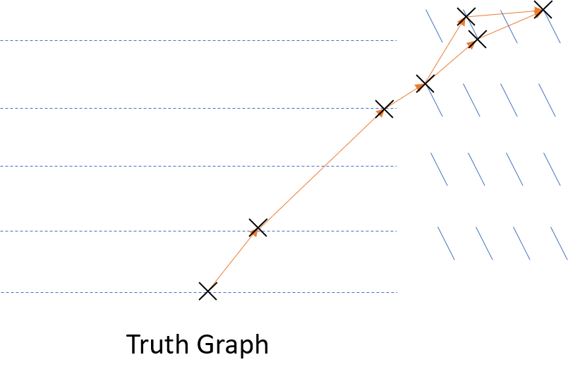
A truth graph is simply some target graph that tries to represent the underlying physics in some way. It must be opinionated, and there is clearly not a single, correct way to define it. That said, for the ITk geometry, we define it by: 1. Order all spacepoints of a track by increasing distance from its creation vertex 2. Connect each pair of spacepoints in this sequence, as an edge in a graph 3. (Module-wise definition) Where two spacepoints are on the same module, do not join them. Instead, form all pair combinations with the preceding and succeeding spacepoints.

To phrase this module-wise defintion differently, for the set of spacepoints {x_i} and modules {m_i} in the diagram, we order all spacepoints as

[(x_0, m_0), (x_1, m_1), (x_2, m_2), (x_3, m_3), ((x_4, x_5), m_4), (x_6, m_5)]

Therefore our edge list becomes

(x_0, x_1), (x_1, x_2), (x_2, x_3), (x_3, x_4), (x_3, x_5), (x_4, x_6), (x_5, x_6)

This is achieved quite efficiently in code with: ``` py title="get_modulewise_edges()" ... signal_list = ( signal.groupby( ["particle_id", "barrel_endcap", "layer_disk", "eta_module", "phi_module"], sort=False, )["hit_id"] .agg(lambda x: list(x)) .groupby(level=0) .agg(lambda x: list(x)) )

true_edges = [] for row in signal_list.values: for i, j in zip(row[:-1], row[1:]): true_edges.extend(list(itertools.product(i, j))) ```

Modulewise and PID Truth

Given these definitions of truth, we can visualize them both on an example graph constructed across two track:

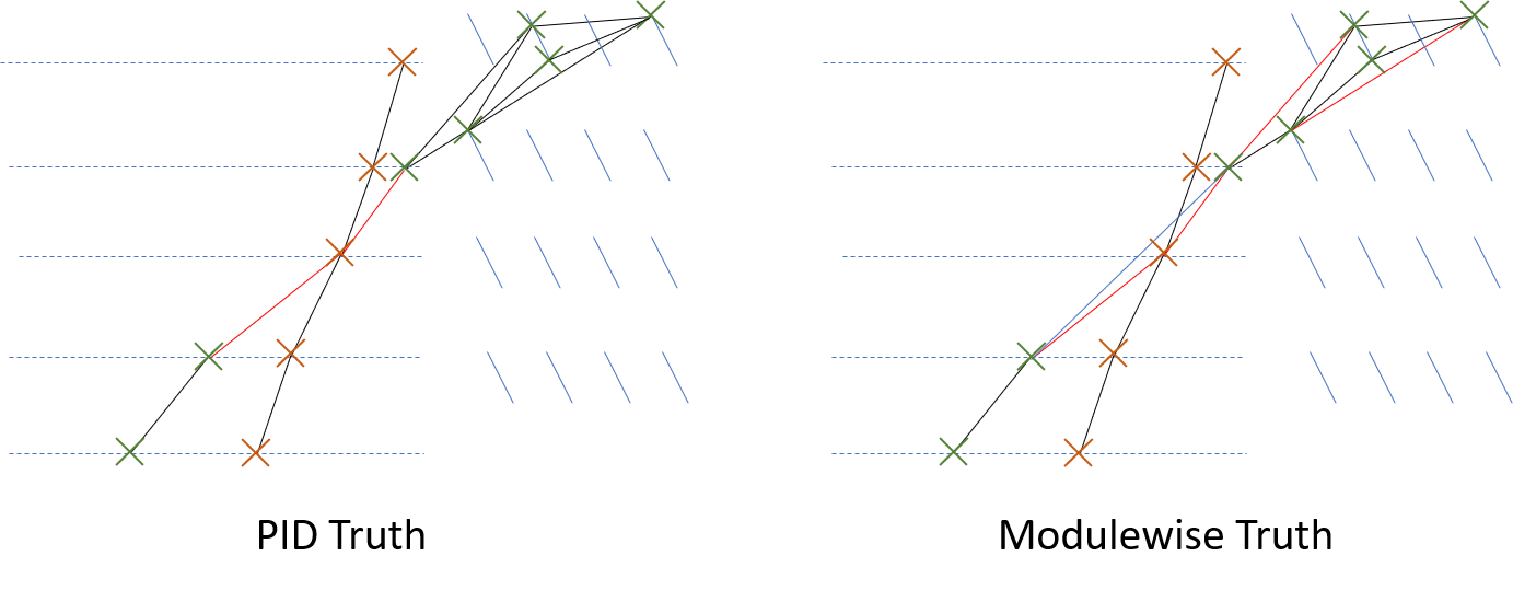
Two graphs with different ground truth definitions for the edges. Black edges are true positives, red a false positives, blue are false negatives

Note that PID truth is fairly obvious: if an edge connects nodes of the same color (i.e. from the same particle) then it's a true positive, otherwise it's a false positive. In the construction of a graph with this definition of truth, there's no real concept of a "missing true edge" - or false negative - since a track of N spacepoints has N choose 2 (O(N^2)) "true edges", which is computationally expensive to handle (see Embedding training to understand why). This is why this definition is not used in graph construction. Once constructed, and each existing edge is being classified, it makes more sense to use this definition.

The modulewise truth takes the graph on the left, but applies our truth graph to it. Thus, we see that edges that skip across the sequence are treated as false. We also see that we can efficiently define false positives, since each particle of N spacepoints will only have O(N) true edges. The trade-off for this more physically-motivated truth definition is that it's more expensive to calculate the accuracy and loss functions. Instead of simply checking the PID, we have to do a graph intersection, which provides a full list of true/fake positive/negative edges in the prediction graph.